enter exponents in Excel

How to Email an Excel attachment From Google Sheets!

By Blog, Video

We’ve all experienced working on Google Drive or Sheets and then needing to send the document to a colleague or friend, only to be stumped by the various drop downs and buttons to look through to figure out how to do what we intend successfully and quickly. So, today I’m going to show you an easy way to convert a Google Sheet to an Excel .xlsx document to email as an attachment.
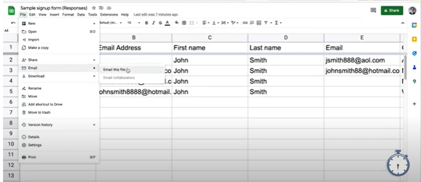
  1. You will want to pull up the Google Sheet you want to send. Here’s how to do it: go to “File”, and then select “Email”.
  2. In the “Email this file” pop up, you will be able to input the receivers name (if their name and email are already in your address book) or their email address. This doesn’t require somebody to have a Google account or that they are a collaborator on the document. So, you can also type in personal email or something else or paste in something.
  3. Also, in the “Email this file” pop up, you can see that the subject is the title of the particular form you’re sending. Then, below that, you put a message about the document or informing your colleague about anything.
  4. Finally, at the very bottom of the pop up, you will change the “File type” from pdf to Microsoft excel. And then click send. The document will send as a .xlsx attachment.

The document can be opened in Google Sheets again, downloaded and opened in Microsoft Excel, or some other program that can read .xlsx files.

For a more visual step by step example, or if you’re just a visual learner, here is my video going through all the steps to email an excel attachment!

If this helped you out, please take a moment to browse my website. Check out my YouTube channel @In30Minutes for other helpful tips and tricks. For more information, you can reference my book about Google Drive that explores docs, sheets, slides, and many other Google apps. It’s currently in its third edition and available on in30minutes.com. Additionally, you can find multiple other guidebooks for any of your other technological needs on the website. We also have cheat sheets for Google sheets, both basic and intermediate level.
How to calculate the yield on a CD in Excel

By Blog, Video

Today I’m going to show you how to calculate the yield and compound interest for a certificate of deposit or a loan with the FV() function in Microsoft Excel. You can find the video explaining this on my YouTube Channel @In30Minutes .

Option 1: Using a Calculator

There are two ways you can calculate yield of a CD. However, the first way you can calculate yield is in a less efficient way by using a calculator.

Let’s say that you have a $10,000 certificate of deposit. What you’ll just do is simple multiplication. Let’s say it has a 2% interest rate. Then you’ll press the equal button ten times, and it’ll give you a value.

The problem with this method is it’s not really calculating interest the way banks calculate interest. It may give you the wrong value not only because it’s not calculating monthly interest, but also because you might press the equal button eleven times or nine times if you’re not being careful.

Option 2: Pasting a Formula into Excel

So, the way that you should do it is by using Excel, which fortunately has a formula that will make it really easy to calculate. It might seem daunting at first, however once you understand the way it works, it’s actually quite easy. Here is the formula: =FV(RATE, NPER, PMT, PV).

Calculate a certificate of deposit’s future value:

  • Use =FV(RATE, NPER, PMT, PV) formula
  • FV is the future value
  • RATE is the interest rate for the period
  • NPER is the number of periods (months, years)
  • PV is the present value or the principal
    • PV is negative to reflect a deposit
  • PMT is zero (no additional payments)

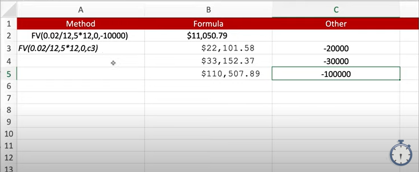
For example, to input yield for $10,000, 5-year CD at 2% interest compounded monthly into the formula would look like: =FV(0.02/12,5*12,0,-10000). So, you can take this formula and paste is in Microsoft Excel, when you press enter it will calculate it automatically. In this case, the final value of account is $11,050.79.

Option 3: Calculating a Column in Excel

Shows how to format Excel to yield and compound interest for a CD

There’s another way you can calculate the yield on a CD using the above formula If you have numbers that are already inserted into a column. Instead of typing in the value into the last place, (PV), of the formula, you would type in the cell of the Excel column.

Then we’re going to just paste that formula and press enter, to give you the final value. You can drag this formula down and press enter to generate the final value of the other numbers in the column.

This is a quick way to calculate the value of a deposit or any other sort of loan, borrowing, or any scenario where you want to calculate the interest on a compounded monthly basis.

If this helped you out, please take a moment to browse my website and check out my YouTube channel @In30Minutes for other helpful tips and tricks. For more information on how to get the most out of excel, check out my book Excel Basics: in 30 Minutes, as well as the Excel cheat sheets that are created with examples like this.

How to join text & values in Microsoft Excel

By Blog, Video

Today I am going to show you a cool trick to use Concatenate to join text and values in Microsoft Excel. To start, I have this simple list of first name, last name, and age. The goal is to be able to paste this into an email, into a word document, or something similar. Instead of just showing the raw data, it would look more like “John Smith is 33 years old.” The excel function that would do this for you is called Concatenate.

In order to join text and numbers, you would use the =CONCATENATE() function. Inside the parenthesis, the referenced cells can contain formulas or other functions. You can add commas or quotation marks to add text or spaces.

For example, the Excel cells we are using are A1 containing the first name, B1 containing the last name, and C1 containing the age. If we input this into the Concatenate() function it would look like this: =CONCATENATE(A1, “ “, B1, “ is ”, C1, “ years old.”). Make sure to account for any spacing that would need to go in between text or values. As you can see between cells A1 and B1 I added a space using quotation marks, which would create a space between the first and last name.

Then you can paste this into the function bar in Excel, and you can see how Excel will select the three cells referenced. Once you hit return, Excel will automatically create the sentence for you. In our example, it will look like “John Smith is 33 years old.”

If you have a list, all you need to do is use auto fill and drag the function down. This will automatically fill out the rest of your list.

You can utilize this in all kinds of situations, whether you want to make something that’s easier to read, or maybe you want to join some values. For more information, you can check out my YouTube video that shows how to use Concatenate.

If this helped you out, please take a moment to browse my website and check out my YouTube channel @In30Minutes for other helpful tips and tricks. For more information on how to get the most out of excel, check out my book Excel Basics: in 30 Minutes, which covers other basic functions of Excel. As well as the Excel cheat sheets and intermediate level cheat sheet which specifically covers Concatenates.

How to edit Excel files in Google Sheets

By Blog, Video

Today I’m going to be talking about how to edit a Microsoft excel .xlsx file in Google Sheets using the Google Chrome browser. You can also check out my video detailing how to do this as well.

Office Editing Extension:

First, you don’t need to convert an Excel file. All you will need is a Google Drive account and to be working in a Chrome browser for Mac or PC. However, you will need to install a special type of extension in the Chrome browser called Office Editing.

In order to install Office Editing, you need to go to Window and then select extension or go to the chrome web store (chrome.google.com) and then search for it. Extensions are like little software programs that you can attach to Google Drive, docs, or Sheets.

Once you have it installed you have to open the excel document from Google Drive. You cannot upload it directly to Google Sheets. If you do try to upload an excel file into Google Sheets, even using the Google Chrome browser, it will automatically convert it into Google Sheets. Sometimes you don’t want to do that because you might need to keep it in excel.

How to edit Excel files:

So, here’s how you edit Excel files. Open a document from Google Drive: go to new, select file upload, then you find your excel document. Once you click open, it will upload the excel document and you will see a green X next to the document which indicates that it’s an Excel document, not Google Sheets.

You can see that all the data is there, and it uses formulas as well as the raw values. However, unlike Excel and Google Sheets, there is no formula bar or options to create new formulas based on the data. The Office compatibility mode for Excel gives you a limited number of options to manipulate the data, but it doesn’t give you the full suite of tools.

So, let’s say I wanted to alter a formula in a certain cell. If you alter the formula is will update the cell. However, some of the functions, when updated, will create a raw number, but in the wrong number format. To fix this you can go to format then choose number format, such as currency and then adjust the decimal places.

Now, once I’ve done that, if I wanted to, I could just download the excel file and then I can email it to somebody. You can find more instruction how to do this in my article How to Email an Excel attachment From Google Sheets. You could also share this with somebody else in Google Sheets. Usually this is useful for simple edits or to make someone check it before its sent somewhere else.

Also, if you do want to get a more full set of features like making charts or accessing the different features that are on the Google Sheets toolbar, you can convert it to Google Sheets. To do this you will go to File then Save as Google sheets.

If this helped you out, please take a moment to browse my website and check out my YouTube channel @In30Minutes for other helpful tips and tricks. For more information on how to get the most out of Google Sheets, check out my book Google Drive & Docs in 30 minutes to learn more about Google Drive, Docs, Sheets, and Slides.

How to calculate monthly mortgage payments in Excel

By Blog, Video

Today we are going to be talking about how to calculate monthly mortgage payments with the PMT() function in Microsoft Excel. So, you have a situation where you need to borrow $200,000 mortgage over 30 years, and then you have to figure out how much you’re going to be paying for. This example shows what the principal owed every year over 30 years.

To calculate this you can use a built in function that excel includes called PMT or =PMT(). In the parentheses, you can input several values—there can be as many as five—but in this case I’m just going to have three. 

Calculate Monthly Loan Payments:

  • Use =PMT(RATE,NPER,PV) formula.
  • RATE is the interest rate for the period.
  • NPER is the number of periods (months, years).
  • PV is the present value or the principal.

Equation One:

For example, the raw formula for a 30-year loan for $200,00 at 5% interest would be expressed as  =PMT(0.00416666,360,200000). Now, the equation looks a little weird because the values don’t look how you would expect, but that’ll be explained below.

RATE equals 0.00416666 because you need to take interest rate and divide it by 12 to account for the monthly basis for which were calculating. So, in this example it would be 5% interest divided by 12 giving us 0.0041666.

Equation Two:

However, there’s actually an easier way to do it. Instead of calculating all the values separately. You can just express this as a fraction. So, for RATE you would input 0.05/12 and the equation would look like =PMT(0.05/12,360,200000). You can also reference another cell to bring that value in.

So, when you paste this formula into Excel, it expresses it as a negative number because this is what you’re paying out. In this example, your monthly payment is $1,073.64.

Equation Three:

The other way you can express this equation is =PMT(0.05/12,30*12,200000). So, this is going to be a little bit different, but the result should be the same. When you paste it into Excel, it just formatted a little bit differently but the result is the same.

The final way you can format this in Excel put a value in another cell. So, say you put $300,000 in another cell, for example cell C4, then you can just replace the $200,000 in the original equation with the cell C4. If you have a list of numbers, you can just drag the formula down and it will automatically calculate the monthly mortgage payments.

Isn’t that a pretty easy way to calculate monthly loan payments instead of trying to do some really complicated formula on your own?

For more information on how to get the most out of excel, check out my Book Excel Basics: in 30 Minutes as well as the Excel Intermediate cheat sheets. If this helped you out, please take a moment to browse my website and check out my YouTube channel @In30Minutes for other helpful tips and tricks, and where you can find a video that shows how to use PMT() function.


Two ways to enter exponents in Microsoft Excel

By Blog, Video

The question I am answering today is how to enter exponents in Excel. For example, how would you get it to calculate two times two times two or two to the third power? You can also find these instructions in a video on my YouTube Channel.

One way you could do it is just do what I just did here: Type equal then two times two times two. You will get the right answer, which is eight.

However, that doesn’t work if you have a really big exponent or numbers that are hard to type in. For instance, two to the 22nd power or two to the 15th power. It would be tedious to continuously have to type that out. Basically, there are two ways you can type out two to the third or any other exponent.

Method #1: use the carat (^) symbol

The first way to enter exponents into Excel is to use the carrot symbol. If you type in two carat three or 2^3 that is the same as telling excel two to the 3rd power.

So, I’m going to paste in 2^3 and then it will calculate it for you.

Method #2: use the POWER() function

The second way it to use the POWER function. The format for this is =POWER and then in parentheses the argument two comma three. So, =POWER(2,3). Now, I’m going to type that out in excel and, again, it will calculate it for you.

Then if you wanted to change things, for example, instead of doing two to the third power, you want to do two to the 10th power. You can go int and remove three with the ten, which gives you 1,024.

For more information on how to get the most out of excel, check out my Book Excel Basics: in 30 Minutes. As well as the Excel Intermediate cheat sheets, which covers exponents and that’s available from in 30 Minutes. If this helped you out, please take a moment to browse my website and check out my YouTube channel @In30Minutes for other helpful tips and tricks.

How to filter text lists to highlight words in Excel

By Blog, Video

Here is a quick tutorial on how to highlight certain terms in a long list in Microsoft Excel. So, say you have a huge list of terms, and you want to highlight certain words in this giant list. That’s more than 100 terms that contain whatever phrase you’re wanting to highlight. You can easily do this using the filter function.

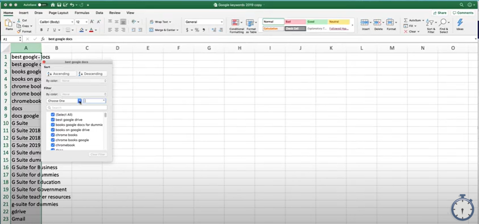
So, you’re going to highlight the column and, either on the Home tab or Data tab, there is a button that says ‘Filter’. Nothing will happen right away; you still have to do a couple more steps. A tiny little downward facing arrow will appear in the first cell of your highlighted column.

filter text lists

When you click on this arrow, a drop-down menu will appear and this will let you set up the filter. Select the ‘Choose One’ drop down, and then select ‘Contains.’ Then in the box to the right of the ‘Choose One’ drop down, input either the word or number that you want to isolate. Then you can clear out of that tab.

As you can see, it basically found all of the terms or cells that have the highlighted term in that giant list.

For more information on how to get the most out of excel, check out my Book Excel Basics: in 30 Minutes. If this helped you out, please take a moment to browse my website and check out my YouTube channel @In30Minutes for other helpful tips and tricks. You can find more on this subject in my YouTube video, Filter text lists to highlight words in Microsoft Excel, that shows how to use the filter function in Excel.

Excel 2019: A quick conditional formatting tutorial

By Video

How to use the conditional formatting tool on the Home ribbon to format text and highlight certain values in an Excel spreadsheet (Excel 2019 for Windows or Excel 2019 for macOS). Length: 4 minutes. Narrator Ian Lamont is the author of EXCEL BASICS IN 30 MINUTES.

Web: https://in30minutes.com/?y
Amazon: https://amzn.to/2DTPiG4
Twitter: https://twitter.com/@in30minutes
Facebook: https://www.facebook.com/in30minutes

DISCLAIMER: This is not an official Microsoft video, nor do I represent Microsoft Corporation. Please review Microsoft’s terms of service before using this feature. i30 Media Corporation cannot be held liable for any direct, indirect, incidental, consequential, or special damages of any kind, or any damages whatsoever, arising out of or in connection with the use of this video.

How to remove duplicate cell values in Excel

By Video

How to remove duplicate text or numerical values in an Excel spreadsheet (Excel 2019 for Windows or Excel 2019 for macOS). Length: 2 minutes. Narrator Ian Lamont is the author of EXCEL BASICS IN 30 MINUTES.

Web: https://in30minutes.com/?y
Amazon: https://amzn.to/2DTPiG4
Twitter: https://twitter.com/@in30minutes
Facebook: https://www.facebook.com/in30minutes

DISCLAIMER: This is not an official Microsoft video, nor do I represent Microsoft Corporation. Please review Microsoft’s terms of service before using this feature. i30 Media Corporation cannot be held liable for any direct, indirect, incidental, consequential, or special damages of any kind, or any damages whatsoever, arising out of or in connection with the use of this video.

How to line up numbers and text in Excel

By Video

How to line up numbers and center text in an Excel spreadsheet (Excel 2019 for Windows or Excel 2019 for macOS). Length: 4 minutes. Narrator Ian Lamont is the author of EXCEL BASICS IN 30 MINUTES.

Web: https://in30minutes.com/?y
Amazon: https://amzn.to/2DTPiG4
Twitter: https://twitter.com/@in30minutes
Facebook: https://www.facebook.com/in30minutes

DISCLAIMER: This is not an official Microsoft video, nor do I represent Microsoft Corporation. Please review Microsoft’s terms of service before using this feature. i30 Media Corporation cannot be held liable for any direct, indirect, incidental, consequential, or special damages of any kind, or any damages whatsoever, arising out of or in connection with the use of this video.